Nonuniformity Correction
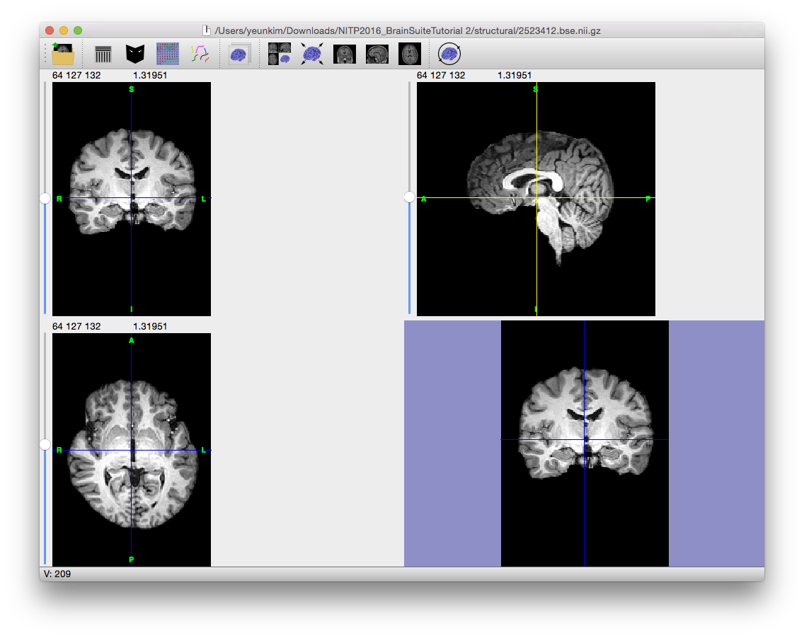
 Magnetic resonance images often exhibit image intensity non-uniformities that are the result of magnetic field variations rather than anatomical differences. These artifacts, often described as shading or bias, can be produced by imperfections in the field coils used in the systems or by magnetic susceptibility changes at the boundaries between anatomical tissue and air. These variations are often seen as a signal gain change that varies slowly spatially. This can result in white matter measurements in one part of the image with the same intensity as grey matter measurements elsewhere; an ideal T1-weighted image would display brighter white matter. This problem can confound tissue classifiers, which often assume that the image intensities of a given type of tissue are relatively uniform throughout the image.
To correct for the gain variation, the Bias Field Corrector (BFC) software is applied. BFC estimates a correction field for the brain region based on a series of local estimates of the tissue gain variation. Initially, BFC computes global tissue values for the mean of white matter, grey matter, and cerebrospinal fluid. This method assumes that all other tissues have been removed.
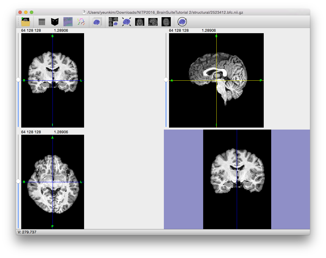
These tissue values are used in a partial volume measurement model that includes a parameter for the local bias effect. By adapting this model to a histogram of a sub-volume of the image, BFC can estimate the gain in this sub-volume relative to the intensities of the entire image. These values are then used to fit a tri-cubic B-spline, which provides an estimate of the non-uniformity. By dividing the original image by this spline, BFC corrects for the non-uniformity field.
As with the BSE dialog, the BFC process can be run in individual steps. However, the intermediate results are not displayed.
The default values for BrainSuite are fairly conservative but typically provide improved tissue classification.
Steps
Initialization
Compute pointwise spline estimates
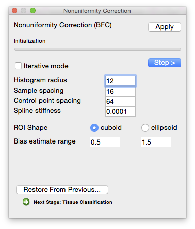
Parameters Histogram radius
- (in voxels—typical range: 8–32)
- The half-width of sub-volume used for sampling, which determines how well-localized the estimate is. A larger radius provides more data to estimate the gain variation, but it also includes a larger area and the gain estimate may not be appropriate for all areas of the sub-volume. A smaller radius will provide a more localized estimate, but has fewer data points to fit. In general, a conservative setting is selected for this value. Increasing the size of the radius will produce smoother estimate fields. Decreasing the value will increase the variations seen in the local gain estimates. It is important to note that the spline-fitting procedure may smooth the field even more.
Sample spacing (in voxels)
- The size of the sample spacing determines how many point estimates are used throughout the image. For smoother gain fields, this value can be increased to produce a sparser sampling. For rapidly changing fields, this number should be decreased to allow more frequent sampling of the gain field.
ROI shape
- Shape of the blocks used for estimating local bias level.
Estimate correction field
Parameters Control point spacing
- Determines how many control points are used in the spline. Larger spacing means fewer points, which allows for fewer bends in the bias field estimate. Smaller spacing allows for more variation.
Spline stiffness
- The spline stiffness parameter influences how much bending is allowed in the gain field of the image. For rapidly varying fields, this parameter should be decreased.
Bias Estimate Range
- An estimate of how much bias the image contains (i.e. how much the intensity value of a tissue type varies across the image relative to its average value). Note that the default values of 0.5 and 1.5 already allow for a very large variation.
Apply correction
Command-Line Usage
usage: bfc -i input -o output [optional settings]
example: bfc -i input_mri.nii.gz -o output_mri.bfc.nii.gz -L 0.5 -U 1.5
Required Settings:
| Flags | Description |
|---|---|
-i <input filename> |
input skull-stripped MRI volume |
-o <output filename> |
output bias-corrected MRI volume |
Optional Settings:
| Flags | Description |
|---|---|
-m <mask filename> |
mask file |
--bias <output filename> |
save bias field estimate |
--maskedbias <output filename> |
save bias field estimate (masked) |
-r <radius> |
histogram radius (voxels) [default: 12] |
-s <spacing> |
bias sample spacing (voxels) [default: 16] |
-c <spacing> |
control point spacing (voxels) [default: 64] |
-w <strength> |
spline stiffness weighting parameter [default: 0.0001] |
--ellipse |
use ellipsoid for ROI histogram |
--block |
use block for ROI histogram |
--iterate |
iterative mode (overrides -r, -s, -c, -w settings) |
--schedule <schedule_file> |
list of parameters in a text file |
--biasprefix <prefix> |
save iterative bias field estimates as <prefix>.n.field.nii.gz |
--prefix <prefix> |
save iterative corrected images as <prefix>.n.bfc.nii.gz |
--extrapolate |
apply correction field to entire volume |
-L <lower> |
minimum allowed bias value [default: 0.5] |
-U <upper> |
maximum allowed bias value [default: 1.5] |
--low |
small bias model [0.95,1.05] |
--medium |
medium bias model [0.90,1.10] |
--high |
high bias model [0.80,1.20] |
--analyze |
generate intermediate files in Analyze format |
--nifti |
generate intermediate files in Nifti format |
--analyzegz |
generate intermediate files in gzipped Analyze format |
--niftigz |
generate intermediate files in gzipped Nifti format |
--eps <epsilon> |
convergence threshold [default: 1e-06] |
--beps <bias_epsilon> |
bias estimate convergence threshold (values > 0.1 disable) [default: 0] |
-v <number> |
verbosity level (0=silent) [default: 1] |
--timer |
display timing information |
Notes:
For anisotropic voxels, distances are scaled based on the smallest dimension. Iterative mode will run multiple passes of BFC using a range of settings to correct for severe artifacts.
Output Files
| Filename | Contents |
|---|---|
| filename_prefix.bfc.nii.gz | Skull-stripped image with bias-field correction applied |

