Tractography Visualization
With the addition of the BrainSuite Diffusion Pipeline (BDP), BrainSuite can process raw diffusion data through distortion correction and anatomical registration to full tractography visualization. BDP handles the distortion correction, ODF (orientation distribution function) and tensor estimation from the command-line (detailed here), while the BrainSuite GUI handles tractography and visualization.
BrainSuite can produce tracks either from ODFs estimated using the Funk-Radon Transformation (FRT) or Funk-Radon and Cosine Transformation (FRACT) for high-direction data sets (usually 40 or more acquired directions), or from tensors for data sets collected with fewer directions.
Generating Tractography
Using FRT/FRACT/3D-SHORE
If BDP was run with the --FRT and/or --FRACT and/or – – 3DSHORE flags, then it will have produced files calculated using FRT in the FRT directory, with FRACT in the FRACT directory and with 3DSHORE in the 3DSHORE directory, respectively. Any of these set of files can be used as needed, though FRACT should provide better angular resolution for single-shell sampled diffusion data and 3DSHORE can be used with multi-shell sampled diffusion data. Each folder contains 45 .nii.gz files and one .odf. This .odf file is a plaintext listing of the .nii.gz files in its folder, and is the file to load into BrainSuite; the .nii.gz files are each one of 45 coefficients to the ODF function.To load the ODF data in BrainSuite, click on File > Open > HARDI SHC Data… (“HARDI SHC” stands for High Angular Resolution Diffusion-weighted Imaging Spherical Harmonic Coefficients).
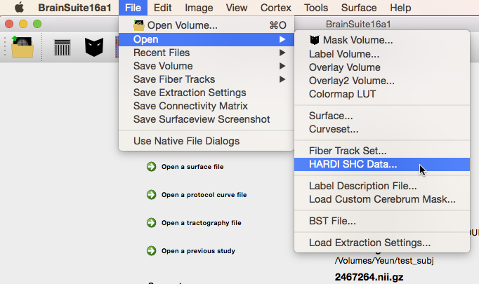
Alternatively, drag the .odf file onto the BrainSuite GUI. The log window will display the names of the files it is opening and, once they have all loaded, appear similar to the image below.
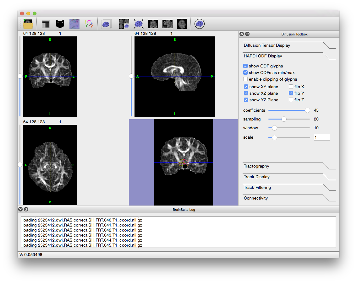
Note that the Diffusion Toolbox opens to the “HARDI ODF Display” tab as well, with settings to control the ODFs’ appearance. Zoom in on the colored area in the surface view to better see the ODF glyphs which represent the orientation of tracts in each voxel. The number of glyphs displayed defaults to a small number to keep the display responsive; moving the “Window” slider in the Diffusion Toolbox will increase the number of glyphs displayed at the cost of decreased responsiveness (i.e. more processing is needed each time you change either the surface or slice views). You can also flip the X, Y, and Z directions as required by your dataset.
BrainSuite can use a mask to contain the tracks it creates, so it is often helpful to load a white matter mask before computing tracks to limit processing time. If the full BrainSuite Cortical Surface Extraction sequence has been run on the anatomical scan, use the inner cortical mask generated after de-wisping (the file ending with .cortex.dewisp.mask.nii.gz). Otherwise (or if that mask requires tweaking), use the mask tool to generate a manual mask. The mask does not need to be exact — it is more important to include white matter than exclude grey matter and CSF.
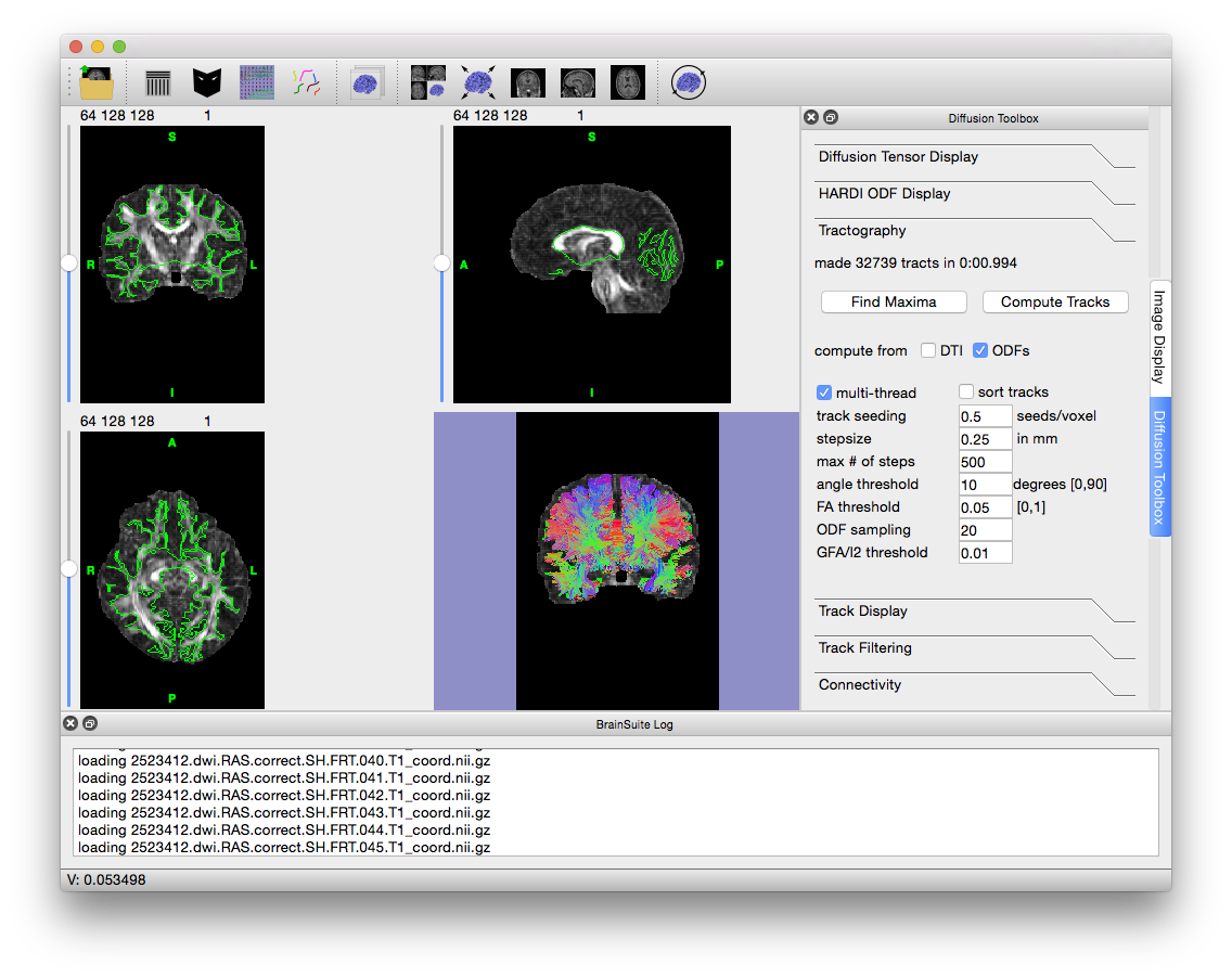
To produce tracks from the loaded ODFs, click on the “Tractography” tab in the Diffusion toolbox. If only the FRT, FRACT or 3DSHORE ODF file has been opened, then “compute from ODFs” should already be checked; if it is not, then select the box and make sure “compute from DTI” is unchecked. Depending on your computer and visualization needs, it may be helpful to decrease “Track Seeding” from its default 1 to 0.5; this will decrease the track density, lowering the amount of memory and processing required for viewing. Click on “Compute Tracks” to create the tracks.
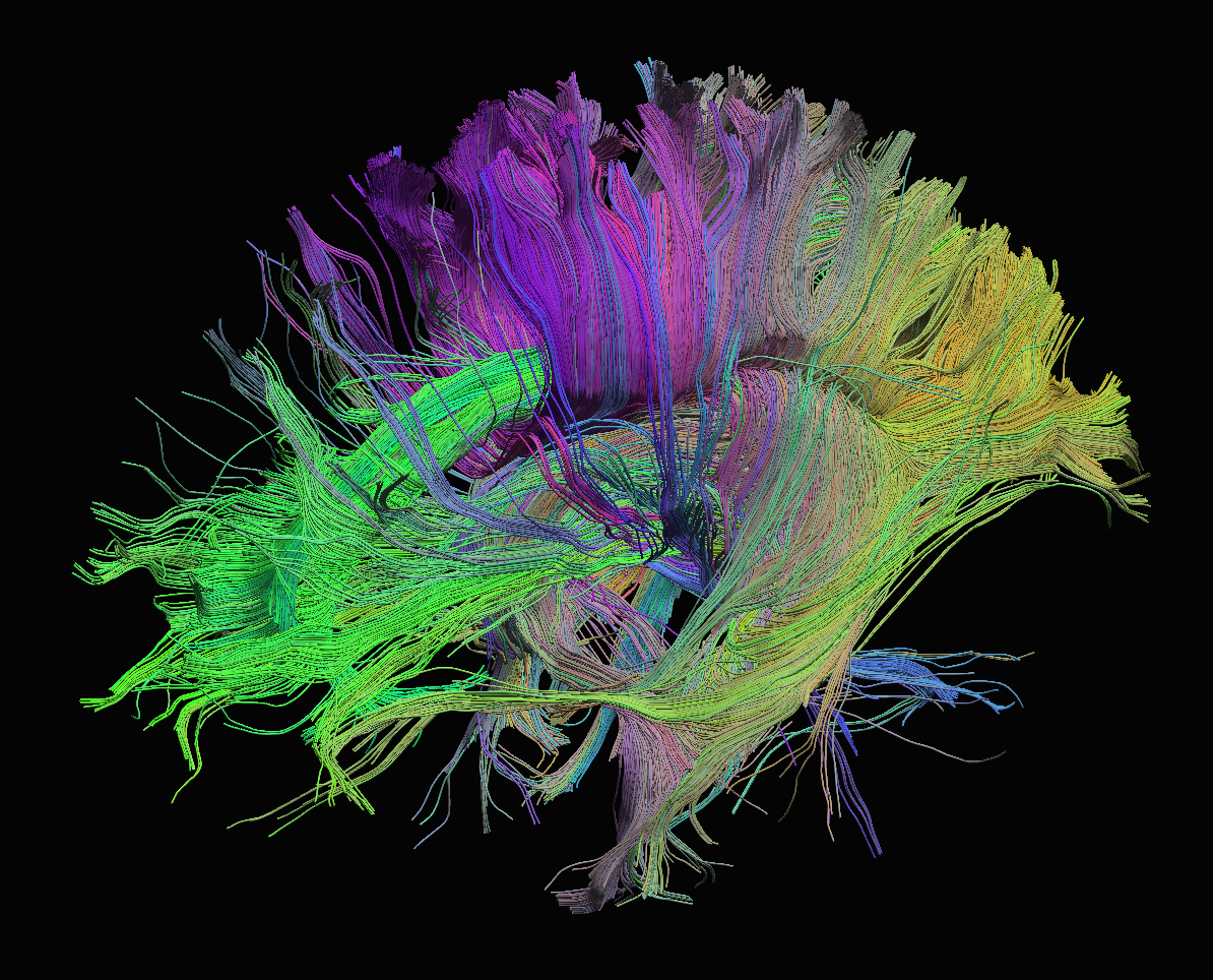
 Tracks generated from FRT ODFs. The white matter mask was generated using thresholding from the Mask tool.
Here you can create the content that will be used within the module.
Using Tensors
If BDP was run with the --tensor flag (or both --FRT (or --FRACT) and --tensor), then it calculated diffusion tensors for the data and saved them in a .eig.nii.gz file. To open them in BrainSuite, just use Open > Open Volume…, or drag the .eig.nii.gz file onto the BrainSuite GUI. It will look similar to the image below.
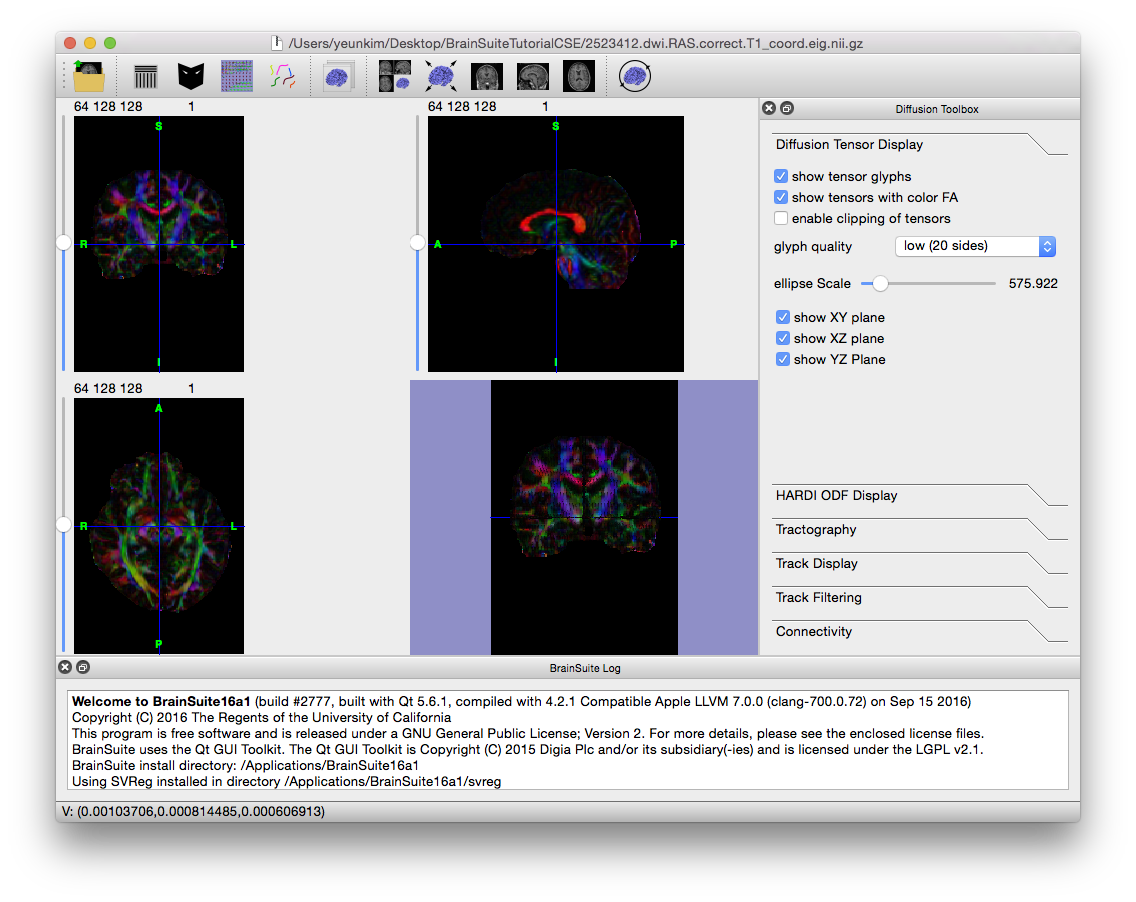
Note that the Diffusion toolbox opened to the “Diffusion Tensor Display” tab as well. Use this to change the display of the tensor ellipsoid glyphs, which can be seen when zooming in on the surface view.
BrainSuite can use a mask to contain the tracks it creates, so it is often helpful to have a white matter mask loaded before computing tracts to limit processing time. If the full BrainSuite Cortical Surface Extraction sequence has been run on the anatomical scan, then use the inner cortical mask generated after de-wisping (the file ending with .cortex.dewisp.mask.nii.gz). Otherwise (or if that mask requires tweaking), use the mask tool to generate a manual mask. Open the anatomical scan and use the threshold level to create a mask, then the dilation and erosion tools and “select foreground” to tweak it as needed, or use the manual brush. The mask doesn’t have to be exact — it is more important to include the white matter than exclude grey matter and CSF.
To produce tracks from the loaded tensors, return to the Diffusion toolbox and click on the “Tractography” tab. If only the .eig.nii.gz file has been opened, then “compute from DTI” should already be checked; if it is not, then select the box and make sure “compute from ODFs” is unchecked. Depending on your computer and visualization needs, it may be helpful to decrease “Track Seeding” from its default 1 to 0.5; this will decrease the track density, lowering the amount of memory and processing required for viewing. Click on “Compute Tracks” to create the tracks.
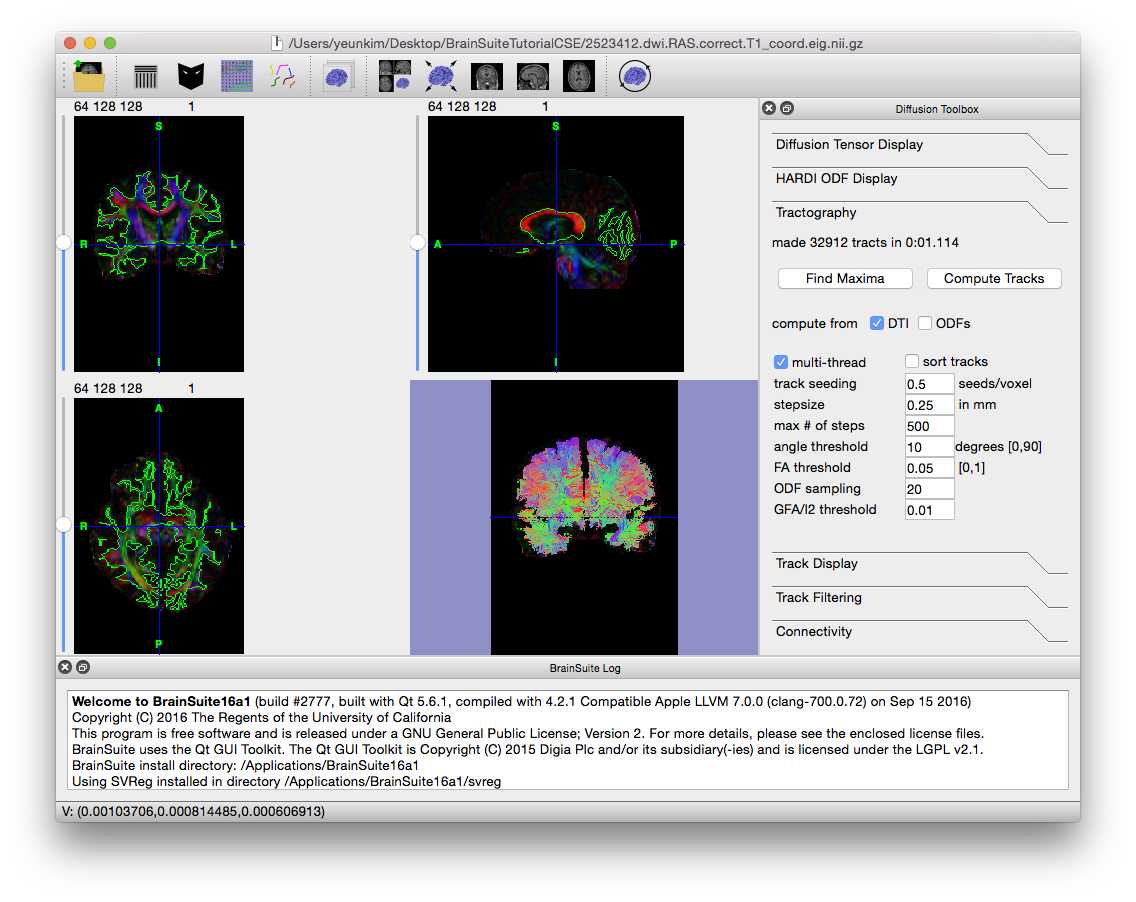 Tracks generated from diffusion tensors. The white matter mask was generated by thresholding the bias-field corrected image, which is also loaded as an overlay volume to make the anatomical features easier to see.