Cortical Surface Extraction
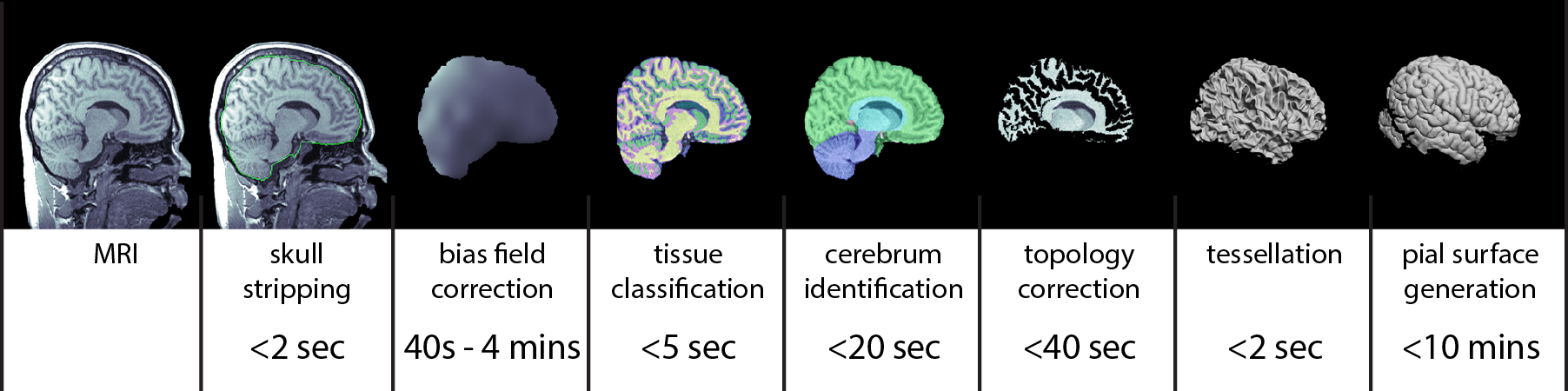
The MRI analysis sequence in BrainSuite produces individual models of brain structures based on T1-weighted MRI of the human head. The models produced include: 1) gross labeling of brain structures (cerebrum, cerebellum, brainstem, ventricles); 2) maps of tissue content in the brain (white matter, grey matter, cerebrospinal fluid (CSF)) at each voxel, including fractional values representing partial volumes; 3) label volumes and surface models of skull and scalp; and 4) models of the inner and outer boundaries of the cerebral cortex. The stages of the BrainSuite extraction workflow are illustrated in the figure above. It can produce a genus zero surface mesh representing the cerebral cortex in ~5 minutes on a 3GHz computer, depending on program settings.
BrainSuite’s Cortical Surface Extraction Sequence can be run using either the program GUI or using the command-line interface as a series of modules. As the GUI calls these same modules, there is no difference in output between using the GUI versus using the command line, provided the same settings are used. For large batch jobs, it is usually helpful to run a few scans through BrainSuite using the GUI to see how the parameters change the output and to determine settings that produce the best results. The rest of the scans can then be run using the command-line modules with those custom parameters.
For information on both the GUI and command-line versions of each stage of cortical surface extraction, click the corresponding link in the following list.
Sequence
- Skull stripping: The procedure begins by removing the skull, scalp and any non-brain tissue from the MRI using a combination of anisotropic diffusion filtering, Marr-Hildredth edge detection, and a sequence of mathematical morphology operators (Sandor and Leahy, 1997; Shattuck et al., 2001).
- Skull and Scalp (Optional): Next, BrainSuite generates 3D surfaces for the skull and scalp, including two layers for the skull, inner and outer, and a rough brain surface.
- Non-uniformity correction: The skull-stripped MRI is then corrected for shading artifacts using BrainSuite’s bias field correction software (BFC; Shattuck et al., 2001). This estimates local gain variation by examining local regions of interest spaced throughout the MRI volume. Within each region, a partial volume measurement model is fitted to the histogram of the region. One component in this model is the gain variation, thus the fitting procedure produces an estimate of the gain variation for that ROI. These gain estimates are then processed to reject poor fits. A tri-cubic B-spline is then fitted to the robust set of local estimates to produce a correction field for the entire brain volume, which is then removed from the image to produce a skull-stripped, nonuniformity corrected MRI.
- Tissue classification: Next, each voxel is classified according to the tissue types present within the extracted brain. The partial volume measurement model is used again, in this case under the assumption that the gain is uniform, and is combined with a spatial prior that models the largely contiguous nature of brain tissue types. This classifier assigns tissue class labels representing white matter, grey matter, and CSF, including pairwise combinations of these; it also estimates fractional measures of grey matter, white matter, and CSF for each voxel (Shattuck et al., 2001).
- Cerebrum labeling: The cerebrum is extracted from the tissue-classified volume by computing an AIR nonlinear registration (Woods et al., 1998) to align a multi-subject atlas average brain image (ICBM452; Rex et al., 2003) to the subject brain image. This atlas has been manually labeled to identify left and right hemispheres, cerebellum, brainstem, and other similarly general areas. The labels are transferred from the atlas space to the individual subject space, allowing BrainSuite to produce a cerebrum-only mask.
- Initial inner cortex mask: These structure labels are combined with tissue fraction maps produced during tissue classification, enabling BrainSuite to create a binary volume representing the voxels of the cerebrum that are interior to the cortical grey matter.
- Mask scrubbing: Segmentation errors due to noise and other image artifacts can lead to rough boundaries on the inner cerebral cortex model. At this stage, a filter is applied to remove some of these surface bumps and pits based on local neighborhood analysis.
- Topology correction: In healthy subjects, assuming the cerebral cortex is closed off at the brainstem, the boundary of the cortex should be topologically equivalent to a sphere, i.e., it should have no holes or handles. However, because of segmentation errors, surfaces that are generated directly from the binary object produced by the previous step are likely to contain topological holes or handles. These can lead to subsequent problems in producing flat-maps or making 1-1 surface correspondences across subjects. Thus, a graph-based algorithm is applied to force the segmented group of voxels to have spherical topology (Shattuck and Leahy, 2001). This method operates by analyzing the connectivity information in each slice of data to produce graph representations of the object and its background. If these graphs are both trees, then the surface has the correct topology. BrainSuite’s algorithm analyzes these graphs using a minimal spanning tree algorithm to identify locations in the brain volume where it can make minor corrections, either adding or removing voxels from the binary object, to enforce the topological rule. The result is a binary object that, when tessellated, will be a genus zero model of the inner cerebral cortex.
- Wisp filter: Even after topology correction, individual voxel misclassifications near the white/grey matter tissue interface appear as bumps or, when they consist of multiple connected voxels, strands or wisps that clearly do not represent true anatomy. These strands introduce sharp features in the surface that are inconsistent with anatomical expectations of smoothness, leading to problems in the formation of the pial surface. To address this, we recently devised a graph-based approach that is similar to our topology analysis code. This new method analyzes the binary segmented object to identify areas corresponding to these strands and then removes them. As this procedure uses the same graph-based representation of the brain volume as the topology correction step, the additional computation cost is only a few seconds. The result is a smoother inner cortical surface mask, which in turn produces improved inner cortical and pial surface models.
- Surface generation: A surface mesh is produced from the binary object using an isocontour method. The boundary of the binary object represents the inner cortical boundary.
- Pial surface generation: This module takes as input the initial mask of the white/grey matter tissue interface and the surface defined by this boundary and generates a surface representing the pial (outer cortical) surface. It also uses a set of tissue fraction values that define how much GM, WM and CSF are contained within each voxel of the brain image. Using an iterative process, each vertex of the WM surface is moved under the influence of several forces: the first pushes the vertex outward along the surface normal, while the others try to maintain the smoothness of the initial surface. The movement of each vertex stops when it moves into a location with a significant CSF component or when its motion would cause the surface to self-intersect. The result is a 1-1 map between the points on the inner cortical surface model and the pial surface model, which can provide a direct estimate of the cortical thickness.
- Hemisphere labeling: Applying the labels produced in step (4), the current step assigns left and right hemisphere labels to the inner cortical surface models, which are then transferred to the corresponding locations on the pial surface models. Each surface is then split into left and right hemispheres.
The complete sequence described above has been developed in C++. It is available as part of the BrainSuite software distribution.