Diffusion Imaging Tutorial
.bvec, and .bval files available here. Unzip them and copy them into the folder you used for the previous exercises. If you haven’t run the previous exercises, then download all of the required files from here and unzip the folder to a convenient location (such as your desktop).The files 2523412.nii.gz, 2523412.dwi.nii.gz, 2523412.dwi.bvec, and 2523412.dwi.bval are part of the Beijing Enhanced dataset, released by Beijing Normal University as part of the International Neuroimaging Datasharing Initiative (INDI) under a Creative Commons Attribution-NonCommerical 3.0 Unported License (CC-BY-NC). More information on the complete dataset is available online here, and it can be downloaded from NITRC.
Process Diffusion Data with BDP
bdp.exe below with bdp.sh.- Open Command Prompt or Terminal. On Windows, search for “Command Prompt” in the Start Menu under All Programs > Accessories. In Mac OS X, look for Terminal in the Utilities directory of your Applications folder or in Launch Pad. In Linux, search for Terminal, often either in your Applications menu or in the right-click context menu. The rest of this tutorial will be written from the perspective of the Window’s Command Prompt, but the commands to enter in Linux and Mac OS X are the same (with
bdp.exeasbdp.sh). - In the terminal/command prompt, navigate to the directory containing the files used in these exercises. For example, for Windows:
cd C:\Users\Joe\Downloads\BrainSuiteTutorialDWI
For Mac/Linux example:
cd /Users/Joe/Downloads/BrainSuiteTutorialDWI - If the BDP script has not been added to your path variable, then replace all instances of “
bdp.exe” with the full path to BDP; “bdp.exe” is located in the bdp folder in BrainSuite16a1 folder (i.e."c:\Program Files\BrainSuite16a1\bdp\bdp.exe").
Type the following into the command line (all on one line) and press enter (if Windows):bdp.exe 2523412.bfc.nii.gz –tensor –FRT –FRACT –nii 2523412.dwi.nii.gz -g 2523412.dwi.bvec -b 2523412.dwi.bvalIf Mac or Linux, then type:
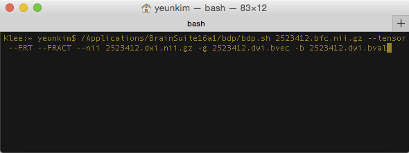
As a command-line program, BDP’s behavior is dictated by input flags. The above command tells BDP to calculate orientation distribution functions and diffusion tensors using the
2523412.dwi.nii.gzdiffusion file, with the gradient directions given in2523412.dwi.bvecand b-values in2523412.dwi.bval. The BFC file is used for registration-based distortion correction and aligns the diffusion data with the anatomical data processed with the cortical surface extraction sequence and SVReg. BDP takes ~1 hour to run, so you can take this time to look over the documentation of the other flags available at BDP’s flag page.
Visualize Fibers in BrainSuite
- Once BDP has finished running, open BrainSuite.
- We will generate tracks from the orientation distribution functions (ODFs) generated via the Funk-Radon Transform (FRT). To do so, open
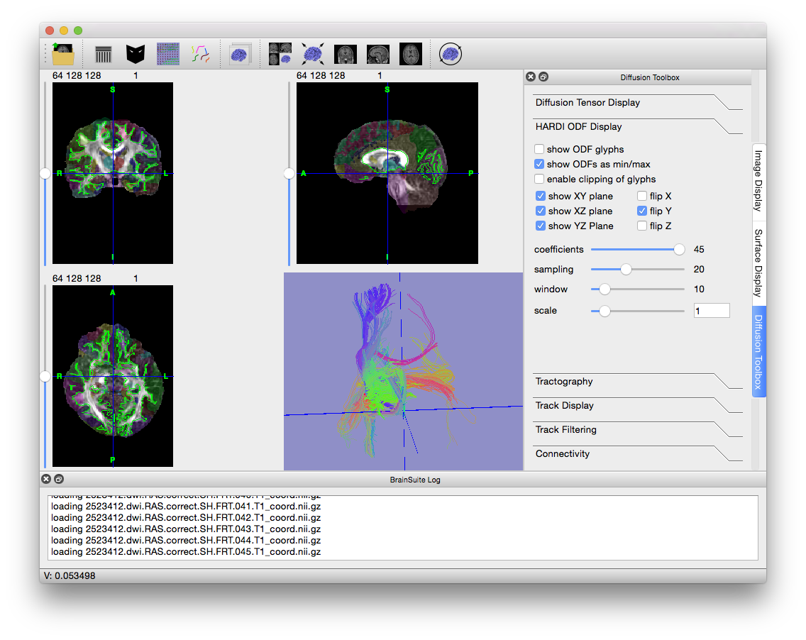
2523412.dwi.RAS.correct.SH.FRT.T1_coord.odf, which BDP created in the FRT folder within the original working directory. To open it, go to File > Open > HARDI SHC Data… and navigate to the FRT folder. - BrainSuite will load the 45 files describing the functions and then display them. If you still have BrainSuite open after running SVReg, then the labels and surfaces generated by SVReg will also be displayed. Otherwise, the window will look like the figure below.
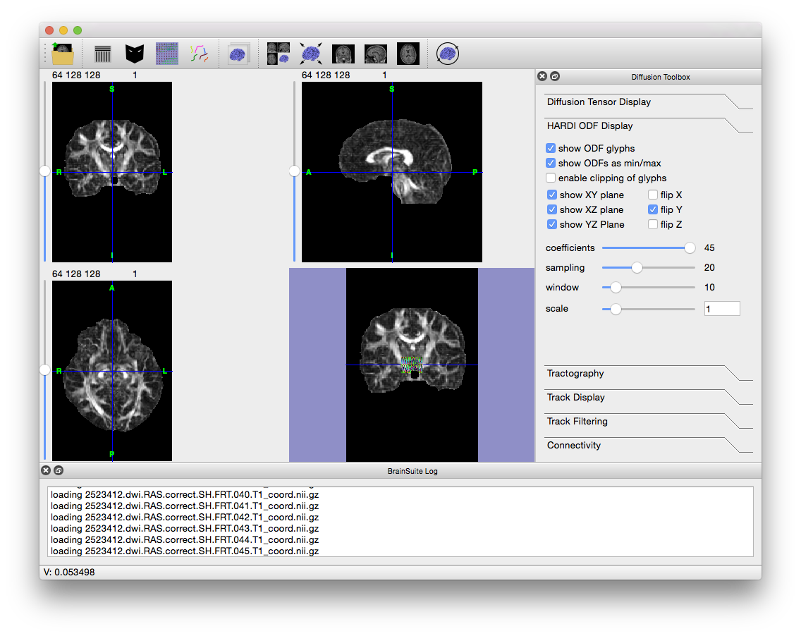
- Note the colored glyphs in the surface view (if you have surfaces open, close them to see the glyphs). These are the ODFs. If you zoom in, you can see that they look like blobs in the shape of the tracks running through them. To see a larger sample, move the Window slider (in the Diffusion toolbox to the right) all the way to the right. Play around with the other settings in the “HARDI ODF Display” tab of the Diffusion Toolbox to see how they affect the visualization. Keeping the window size small will keep the surface view responsive. Once you are done, uncheck “Show ODF glyphs”.
- To produce tracks, open the “Tractography” tab of the Diffusion toolbox. To generate lower-quality tracks that are easier to explore, change the value in “Track seeding” from 1 to 0.5 to decrease the number of tracks produced, requiring less processing and memory. Lowering this value is useful in generating “example” tracks before running higher quality, more intensive processing.
- If a mask is loaded, BrainSuite will only compute tracks within that mask. Again, to speed up processing and reduce the memory requirements, load the inner cortical mask generated during the CSE process. Go to File > Open > Mask Volume…, navigate to the folder with the tutorial files, and load
2523412.cortex.dewisp.mask.nii.gz. However, if you would like to process the tracts within the medulla, i.e. corticospinal tract, you can load the brain mask (2523412.mask.nii.gz) to do so. - Make sure that “compute from ODFs” is checked and then hit “Compute Tracks”. Once the tracks have been computed, your screen should look like the image below.
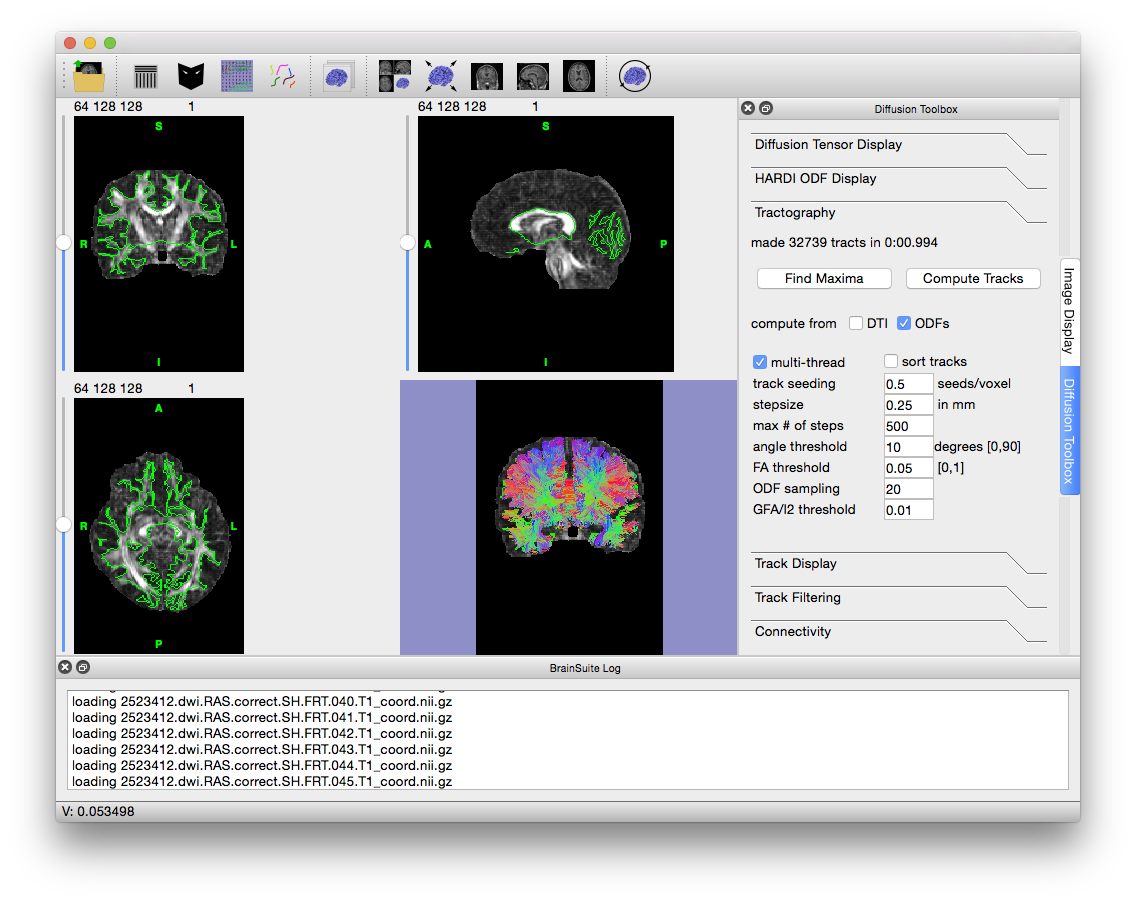
- Press Ctrl + V to hide the slices in the surface view and get a better look at the fiber tracks. Try out the options in the Track Display and Track Filtering tabs to see how they change the display of the tracks (changing “length thresh” in the “Track Filtering” tab to 15 often results in nicer images).
Calculate Connectivity
- To combine these tracks with the labels from SVReg and compute the connectivity between regions, load the SVReg ROI labels. Go to File > Open > Label Volume… and open
2523412.svreg.label.nii.gz. - Click on the “Connectivity” tab of the Diffusion toolbox and then click “Compute Connectivity”. After a short pause, a circle graph like the one below will appear.
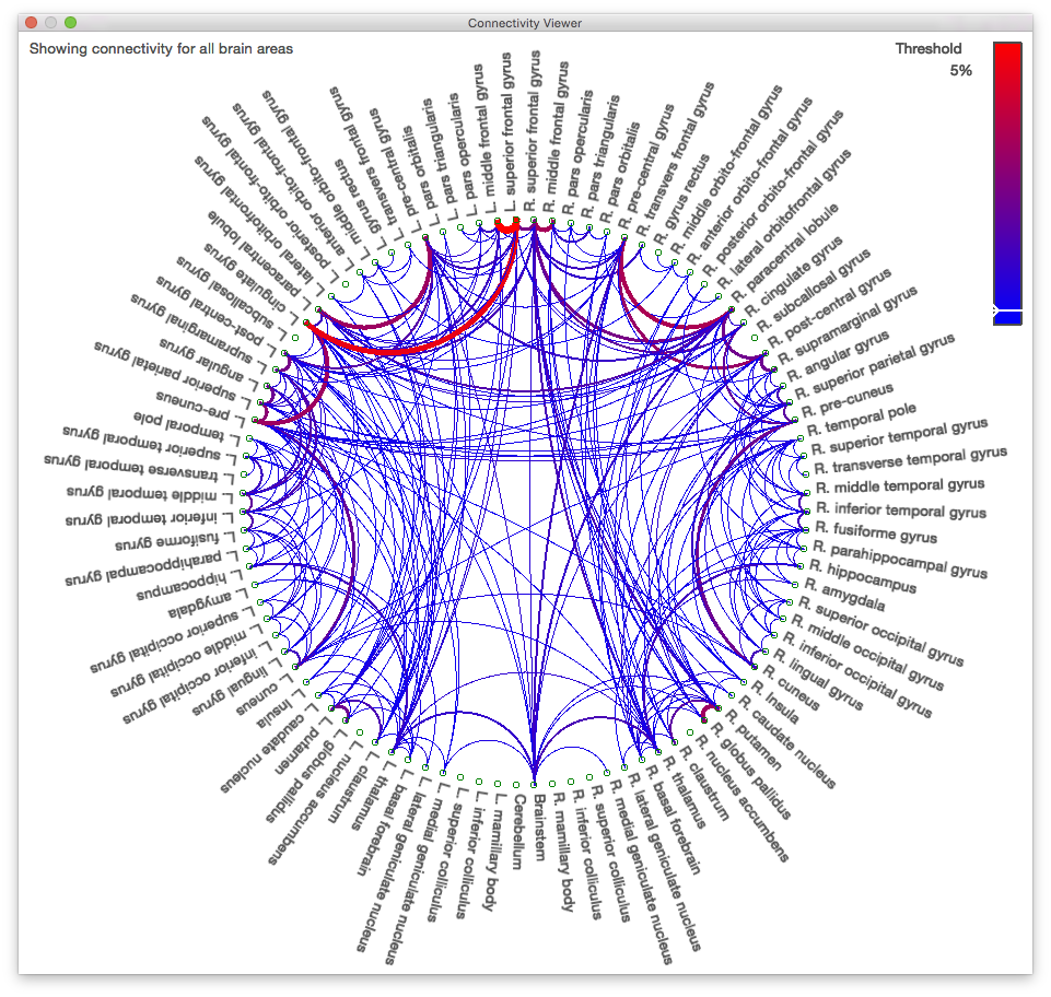

Due to the mask we used and the default threshold of 5% on the graph, some areas may look like they are not connected to anything else. Lowering the threshold or running the tractography process without a mask would fill in these connections.
- Click on “R. thalamus” near the bottom of the graph. Notice that the connectivity viewer updates to show only the connections of the right thalamus. Also, note that the surface view changed to display only those tracks that pass through the right thalamus.
- Hold down Shift and click on “L. thalamus”. Now the graph shows the connections of both thalami, and the surface view shows the tracks passing through both.
- Click on “R. thalamus” again to show only its connections, then hold down Ctrl and click on “R. putamen”. Now the graph displays only the connection between these two regions, and the surface view updates to show only tracks that pass through both.