Quick Start: Diffusion Imaging
BrainSuite includes tools for aligning diffusion data with structural scans, which, when coupled with the labeling provided by SVReg, allows for analysis such as automatic processing of the connectivity between regions of interest. The minimum files required for BrainSuite Diffusion Pipeline (BDP) are the diffusion data and the bias-field corrected image generated by BrainSuite’s Cortical Surface Extraction Sequence.
More detailed information about BDP is available in the Processing section of this site, but the steps below can get you started.
Process Diffusion Data with BDP
BDP is a command-line only program. Open a terminal (or Command Prompt on Windows) and run the following command. A screenshot of the command prompt (on Windows) is also shown below.
Windows:
bdp.exe 2467264.bfc.nii.gz --tensor --FRT --FRACT --nii 2467264.dwi.nii.gz -g 2467264.dwi.bvec -b 2467264.dwi.bvalLinux and Macintosh:
bdp.sh 2467264.bfc.nii.gz --tensor --FRT --FRACT --nii 2467264.dwi.nii.gz -g 2467264.dwi.bvec -b 2467264.dwi.bval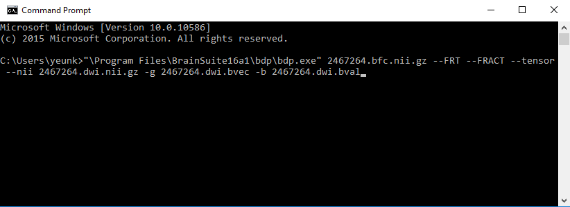
Visualize Streamline Tractography in BrainSuite
BDP’s output files can be loaded into BrainSuite for visualization (e.g., colored fractional anisotropy) or for streamline tractography. Streamline can be created from these files (in order of increasing angular resolution):
fileprefix.dwi.RAS.correct.T1_coord.eig.nii.gz(diffusion tensors)fileprefix.dwi.RAS.correct.SH.FRT.T1_coord.odf(located in the FRT folder when ODFs are calculated)fileprefix.dwi.RAS.correct.SH.FRACT.T1_coord.odf(located in the FRACT folder when ODFs are calculated)
Load either the .eig.nii.gz file via File > Open Volume… or the .odf file of your choice via File > Open > HARDI SHC Data… (“HARDI SHC” stands for High Angular Resolution Diffusion Imaging Spherical Harmonic Coefficient). The Diffusion Toolbox will open as well.

Click on the “Tractography” tab in the Diffusion toolbox to open it. When using diffusion tensors to create tracks, make sure that “compute from DTI” is checked; when using either of the ODF files, make sure that “compute from ODFs” is checked. Click “Compute Tracks” to produce the fiber tracks.

Calculate Connectivity
You can use the volume labels generated by SVReg with the fibers generated above to explore the connectivity of different brain regions. Go to File > Open > Label Volume… and load fileprefix.svreg.label.nii.gz. Next, open the “Connectivity” tab of the Diffusion toolbox and click “Compute Connectivity.” After a few moments of calculation, a circle graph will appear, displaying connectivity between all brain regions.
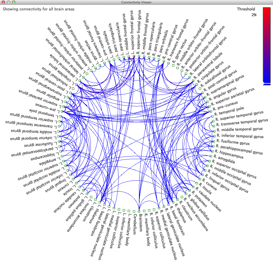
Clicking on a region name in the graph will update the surface view to only show those fibers passing through that area; clicking another label while holding down the Ctrl (Cmd on Mac OS X) will display the fibers connecting those brain regions, while holding down Shift and clicking on additional regions will add the fibers passing through them to the surface view. Keyboard shortcuts for filtering the labels shown are:
| Connectivity Viewer | |
|---|---|
| Key | Action |
| 1 | Show Connectivity for Cortical Areas |
| 2 | Show Connectivity for Frontal Lobe |
| 3 | Show Connectivity for Parietal Lobe |
| 4 | Show Connectivity for Temporal Lobe |
| 5 | Show Connectivity for Occipital Lobe |
| 6 | Show Connectivity for Subcortical Areas |
| 7 | Show Connectivity for Brain Areas |
| 8 | Show Connectivity for All Labeled Regions (includes white matter, ventricles, etc). |